Introductory Statistics: Concepts, Models, and Applications
David W. Stockburger
If a student, upon viewing a recently returned test, found that he or she had made a score of 33, would that be a good score or a poor score? Based only on the information given, it would be impossible to tell. The 33 could be out of 35 possible questions and be the highest score in the class, or it could be out of 100 possible points and be the lowest score, or anywhere in between. The score that is given is called a raw score. The purpose of this chapter is to describe procedures to transform raw scores into transformed scores.
Transforming scores from raw scores into transformed scores has two purposes: 1) It gives meaning to the scores and allows some kind of interpretation of the scores, 2) It allows direct comparison of two scores. For example, a score of 33 on the first test might not mean the same thing as a score of 33 on the second test.
The transformations discussed in this section belong to two general types; percentile ranks and linear transformations. Percentile ranks are advantageous in that the average person has an easier time understanding and interpreting their meaning. However, percentile ranks also have a rather unfortunate statistical property which makes their use generally unacceptable among the statistically sophisticated. Each will now be discussed in turn.
A percentile rank is the percentage of scores that fall below a given score. For example, a raw score of 33 on a test might be transformed into a percentile rank of 98 and interpreted as "You did better than 98% of the students who took this test." In that case the student would feel pretty good about the test. If, on the other hand, a percentile rank of 3 was obtained, the student might wonder what he or she was doing wrong.
The procedure for finding the percentile rank is as follows. First, rank order the scores from lowest to highest. Next, for each different score, add the percentage of scores that fall below the score to one-half the percentage of scores that fall at the score. The result is the percentile rank for that score.
It's actually easier to demonstrate and perform the procedure than it sounds. For example, suppose the obtained scores from 11 students were:
|
33 |
28 |
29 |
37 |
31 |
33 |
25 |
33 |
29 |
32 |
35 |
The first step would be to rank order the scores from lowest to highest.
|
25 |
28 |
29 |
29 |
31 |
32 |
33 |
33 |
33 |
35 |
37 |
Computing the percentage falling below a score of 31, for example, gives the value 4/11 = .364 or 36.4%. The four in the numerator reflects that four scores (25, 28, 29, and 29) were less than 31. The 11 in the denominator is N, or the number of scores. The percentage falling at a score of 31 would be 1/11 = .0909 or 9.09%. The numerator being the number of scores with a value of 31 and the denominator again being the number of scores. One-half of 9.09 would be 4.55. Adding the percentage below to one-half the percentage within would yield a percentile rank of 36.4 + 4.55 or 40.95%.
Similarly, for a score of 33, the percentile rank would be computed by adding the percentage below (6/11=.5454 or 54.54%) to one-half the percentage within ( 1/2 * 3/11 = .1364 or 13.64%), producing a percentile rank of 69.18%. The 6 in the numerator of percentage below indicates that 6 scores were smaller than a score of 33, while the 3 in the percentage within indicates that 3 scores had the value 33. All three scores of 33 would have the same percentile rank of 68.18%.
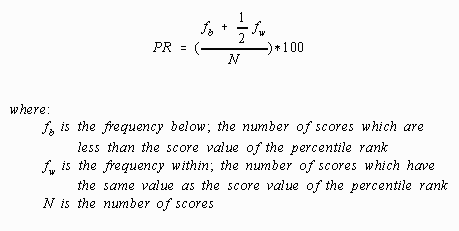
The preceding procedure can be described in an algebraic expression as follows:

Application of this algebraic procedure to the score values of 31 and 33 would give the following results:


Note that these results are within rounding error of the percentile rank computed earlier using the procedure described in words.
When computing the percentile rank for the smallest score, the frequency below is zero (0), because no scores are smaller than it. Using the formula to compute the percentile rank of the score of 25:

Computing the percentile rank for the largest score, 37, gives:

In the last two cases it has been demonstrated that a score may never have a percentile rank equal to or less than zero or equal to or greater than 100. Percentile ranks may be closer to zero or one hundred than those obtained if the number of scores was increased.
The percentile ranks for all the scores in the example data may be computed as follows:
|
25 |
28 |
29 |
29 |
31 |
32 |
33 |
33 |
33 |
35 |
37 |
|
4.6 |
13.6 |
27.3 |
27.3 |
40.9 |
50 |
68.2 |
68.2 |
68.2 |
86.4 |
95.4 |
Although the computation of percentile ranks based on a sample using SPSS is not exactly direct, the steps are relatively straightforward. First, enter the scores as a data file. The data used in the above example is illustrated below.
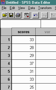
Next, sort the data from lowest to highest.
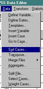
This ranks the scores from lowest to highest as follows.
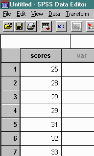
Use the TRANSFORM and RANK options as follows.

The results of the preceding operation appear as a new variable with the same name as the original variable except it begins with an "r". For example, the original variable was named "scores" and the new variable appears as "rscores".
In order to compute percentile ranks as described in the earlier section, a new variable must be created using the COMPUTE command. The new variable is constructed by subtracting .5 from the new rank variable and dividing the result by N. In the example below the new variable is titled "prsamp" and it is computed by subtracting .5 from "rscores" and dividing the result by 11, the number of scores.
The student should verify that the values of the new variable are within rounding error of those in the table presented earlier in this chapter.
The percent of area below a score on a normal curve with a given mu and sigma provides an estimate of the percentile rank of a score. The mean and standard deviation of the sample estimate the values of mu and sigma. Percentile ranks can be found using the Normal Curve Area program by entering the mean, standard deviation, and score in the mu, sigma, and score boxes of the normal curve area program.
|
25 |
28 |
29 |
29 |
31 |
32 |
33 |
33 |
33 |
35 |
37 |
In the example raw scores given above, the sample mean is 31.364 and the sample standard deviation is 3.414. Entering the appropriate values in the normal curve area program for a score of 29 in the Normal Curve Area program would yield a percentile rank based on the normal curve of 24% as demonstrated below.
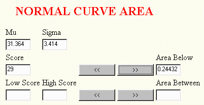
Percentile ranks based on normal curve area for all the example scores are presented in the table below.
|
25 |
28 |
29 |
29 |
31 |
32 |
33 |
33 |
33 |
35 |
37 |
|
3 |
16 |
24 |
24 |
46 |
57 |
68 |
68 |
68 |
86 |
95 |
Percentile ranks based on normal area can be computed using SPSS by using the "Compute Variable" option under the "Transform" command. The "CDFNORM" function returns the area below the standard normal curve. In the following example, "x" is the name of the variable describing the raw scores and "PRnorma" is a new variable created by the "Compute Variable" command. The name "PRnorma" was chosen as a shortened form of "Percentile Rank Normal Scores," the longer name being appropriate for a variable label. In the parentheses following the CDFNORM name is an algebraic expression of the form ( Variable Name - Mean)/Standard Deviation. In the case of the example data, the variable was named "x", the mean was 31.364, and the standard deviation was 3.414. The resulting expression becomes "(x-31.364)/3.414".

This command would create a new variable called "PRnorma" to be included in the data table.
The astute student will observe that the percentile ranks obtained in this manner are somewhat different from those obtained using the procedure described in an earlier section. That is because the two procedures give percentile ranks that are interpreted somewhat differently.
|
Raw Score |
25 |
28 |
29 |
29 |
31 |
32 |
33 |
33 |
33 |
35 |
37 |
|
Sample %ile |
4.6 |
13.6 |
27.3 |
27.3 |
40.9 |
50 |
68.2 |
68.2 |
68.2 |
86.4 |
95.4 |
|
Normal Area %ile |
3 |
16 |
24 |
24 |
46 |
57 |
68 |
68 |
68 |
86 |
95 |
The percentile rank based on the sample describes where a score falls relative to the scores in the sample distribution. That is, if a score has a percentile rank of 34 using this procedure, then it can be said that 34% of the scores in the sample distribution fall below it.
The percentile rank based on the normal curve, on the other hand, describes where the score falls relative to a hypothetical model of a distribution. That is a score with a percentile rank of 34 using the normal curve says that 34% of an infinite number of scores obtained using a similar method will fall below that score. The additional power of this last statement is not bought without cost, however, in that the assumption must be made that the normal curve is an accurate model of the sample distribution, and that the sample mean and standard deviation are accurate estimates of the model parameters mu and sigma. If one is willing to buy these assumptions, then the percentile rank based on normal area describes the relative standing of a score within an infinite population of scores.
Percentile ranks, as the name implies, is a system of ranking. Using the system destroys the interval property of the measurement system. That is, if the scores could be assumed to have the interval property before they were transformed, they would not have the property after transformation. The interval property is critical to interpret most of the statistics described in this text, i.e. mean, mode, median, standard deviation, variance, and range, thus transformation to percentile ranks does not permit meaningful analysis of the transformed scores.
If an additional assumption of an underlying normal distribution is made, not only do percentile ranks destroy the interval property, but they also destroy the information in a particular manner. If the scores are distributed normally then percentile ranks underestimate large differences in the tails of the distribution and overestimate small differences in the middle of the distribution. This is most easily understood in an illustration:
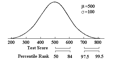
In the above illustration two standardized achievement tests with m =500 and d =100 were given. In the first, an English test, Suzy made a score of 500 and Johnny made a score of 600, thus there was a one hundred point difference between their raw scores. On the second, a Math test, Suzy made a score of 800 and Johnny made a score of 700, again a one hundred point difference in raw scores. It can be said then, that the differences on the scores on the two tests were equal, one hundred points each.
When converted to percentile ranks, however, the differences are no longer equal. On the English test Suzy receives a percentile rank of 50 while Johnny gets an 84, a difference of 34 percentile rank points. On the Math test, Johnny's score is transformed to a percentile rank of 97.5 while Suzy's percentile rank is 99.5, a difference of only two percentile rank points.
It can be seen, then, that a percentile rank has a different meaning depending upon whether it occurs in the middle of the distribution or the tails of a normal distribution. Differences in the middle of the distribution are magnified, differences in the tails are minimized.
The unfortunate property destroying the interval property precludes the use of percentile ranks by sophisticated statisticians. Percentile ranks will remain in widespread use in order to interpret scores to the layman, but the statistician must help in emphasizing and interpreting scores. Because of this unfortunate property, a different type of transformation is needed, one which does not destroy the interval property. This leads directly into the next topic; that of linear transformations.